When solving polynomial equations, it is natural to ask whether solutions always exist. A quadratic can be managed with the quadratic formula, but sometimes the square root is negative, leading into the imaginary and toward the larger complex number system. This shift from real numbers to complex numbers raises a deeper question: does every polynomial of degree greater than zero truly have a root, whether real or complex?
That question lies at the heart of the Fundamental Theorem of Algebra. The theorem connects algebra with the geometry of the complex plane, assuring us that every non-constant polynomial with real or complex coefficients has at least one complex root, and in fact, every polynomial of degree n has exactly n roots.
The effort to prove the theorem shaped the history of mathematics. From Gauss’s first proof to Argand’s proof and later developments in complex analysis, each step strengthened its role as a cornerstone of mathematical thought.
What Is the Fundamental Theorem of Algebra?
The Fundamental Theorem of Algebra states that every non-zero polynomial equation of degree n has exactly n roots in the complex number system, counted with multiplicity. In other words, every polynomial with real coefficients or complex coefficients has a solution. Some of these solutions are real roots, others are imaginary or complex, but none are left unresolved.
A polynomial’s degree is simply its highest exponent, and its roots are the values that make the polynomial equal to zero. Multiplicity accounts for repeated roots. For example, the quadratic equation x² + 1 = 0 has no real root, yet applying the quadratic formula reveals two complex conjugate solutions: i and –i. This shows how polynomials of the form we meet in algebra always resolve into real or complex answers, which is exactly what the theorem guarantees.
Why the Fundamental Theorem of Algebra Matters
The theorem does more than describe roots. It establishes a foundation that connects algebra and complex analysis, showing that every polynomial of degree n has solutions across the entire complex plane.
| Field | Role of the Theorem |
|---|---|
| Algebra | Ensures that polynomials have roots, even when no real root exists. This supports foundational work in elementary algebra and linear algebra. |
| Helps explain the behavior of real and complex solutions using tools like the complex conjugate root theorem. | |
| Applies to polynomials with real coefficients or complex coefficients, confirming that their roots can be real or complex. | |
|
Complex Analysis | The proof of the theorem often relies on applying Liouville’s Theorem across the entire complex plane. |
| Involves topological reasoning and the structure of the complex number system to establish that a complex polynomial of degree n must have roots. | |
| Highlights the deep connection between algebra and complex methods, especially in advanced mathematics and modern proof strategies. |
Historical and Mathematical Significance
Carl Friedrich Gauss gave his first proof in 1799, followed by Argand’s proof in 1806. Later, rigorous proof of the theorem drew on Liouville’s Theorem, calculus, and topological reasoning. Each proof reinforced the idea that polynomials have roots, securing the theorem’s place as a cornerstone in the history of mathematics.
Finding Real Roots Using Graphs and Tables
To start, let’s look at a simple real polynomial:
Example:
f(x)=x3−6×2+11x−6f(x) = x^3 – 6x^2 + 11x – 6f(x)=x3−6×2+11x−6
1.
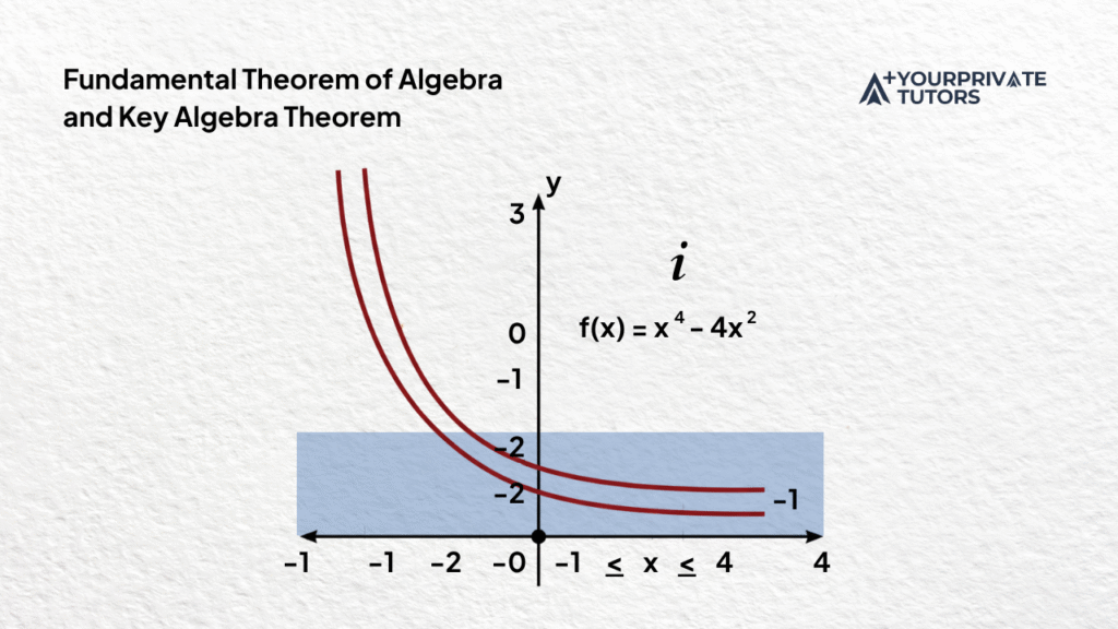
The curve crosses the x-axis at three points: x=1,2,3x = 1, 2, 3x=1,2,3.
- These crossings suggest possible real roots.
2. Check with a table:
| x | f(x) |
|---|---|
| 0 | -6 |
| 1 | 0 |
| 2 | 0 |
| 3 | 0 |
| 4 | 6 |
This table shows that f(x)=0f(x) = 0f(x)=0 at x=1x = 1x=1, x=2x = 2x=2, and x=3x = 3x=3. These values confirm the real roots of the polynomial, matching what we saw on the graph.
3. Confirm.
Substituting shows f(1)=0f(1) = 0f(1)=0, f(2)=0f(2) = 0f(2)=0, and f(3)=0f(3) = 0f(3)=0.
This is a simple proof that the theorem states correctly: a polynomial of degree three has exactly three roots. By the intermediate value theorem, we often expect at least one crossing for real polynomials of odd degree, but here we see all three.
History connection: Argand in 1806 used a geometric approach to prove the fundamental theorem, showing that every complex polynomial of degree n must have roots in the plane.
Using the Factor Theorem to Break Down Polynomials
Now let’s factor f(x)f(x)f(x).
- Since f(1)=0f(1) = 0f(1)=0, the Factor Theorem tells us (x−1)(x – 1)(x−1) is a factor.
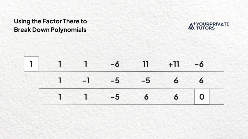
Result: The quotient is x² – 5x + 6, and the reminder is 0. So, f(x) = (x-1)(x² -5x+6).
f(x)=(x−1)(x2−5x+6)f(x) = (x – 1)(x^2 – 5x + 6)f(x)=(x−1)(x2−5x+6)
- Next, factor the quadratic:
x2−5x+6=(x−2)(x−3)x^2 – 5x + 6 = (x – 2)(x – 3)x2−5x+6=(x−2)(x−3)
So the complete factorization is:
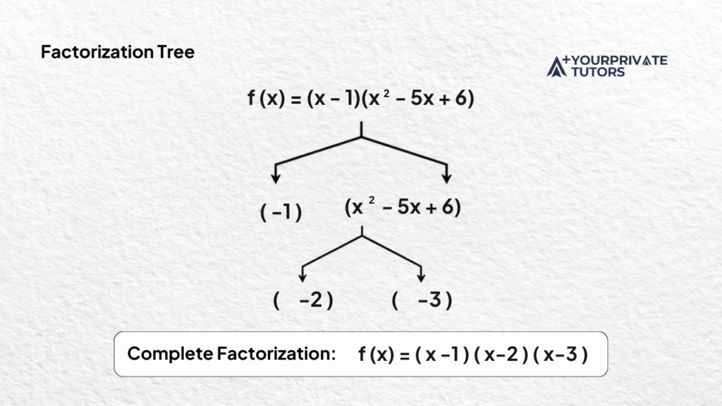
This matches our graph and table. Using the fundamental theorem, we know a polynomial with real coefficients or complex coefficients always resolves into roots — sometimes neat integers, other times messy or complex.
Quick link: Proofs of the fundamental theorem often use algebraic proof or calculus, but this kind of step-by-step factorization is the most hands-on.
What Happens When Roots Aren’t Real?
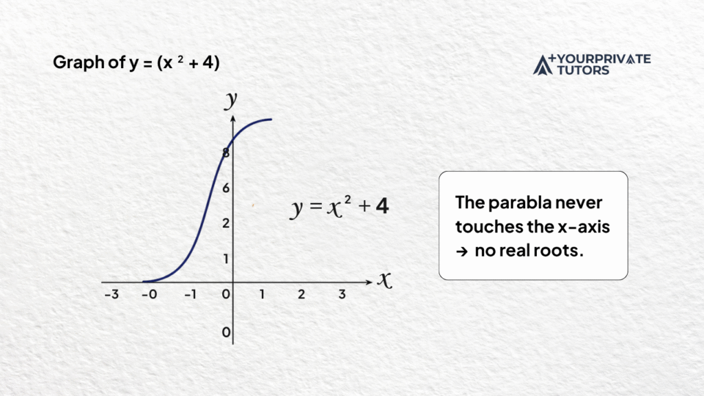
Consider a quadratic complex polynomial:
f(x)=x2+4f(x) = x^2 + 4f(x)=x2+4
1.
2. Check a table:
| x | f(x) |
|---|---|
| -2 | 8 |
| -1 | 5 |
| 0 | 4 |
| 1 | 5 |
| 2 | 8 |
Every value is positive, so the polynomial never equals zero on the real line.
3. Use the quadratic formula:
x=−0±02−4(1)(4)2(1)=±2ix = \frac{-0 \pm \sqrt{0^2 – 4(1)(4)}}{2(1)} = \pm 2ix=2(1)−0±02−4(1)(4)=±2i
So the roots are 2i2i2i and −2i-2i−2i.
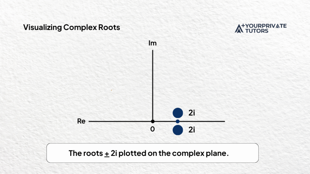
This illustrates what the theorem states: even when graphs show no intercepts, there exists a complex number that makes the polynomial equal to zero.
History connection: Argand’s proof in 1806 and Gauss’s algebraic proof both showed that every complex polynomial of degree n has a root somewhere in the plane. Modern proofs often involve applying Liouville’s Theorem or even topological arguments like the Gauss–Bonnet theorem.
Example: Factoring with Complex Roots
Let’s finish with a quartic that has no real roots:
f(x)=x4+5×2+6f(x) = x^4 + 5x^2 + 6f(x)=x4+5×2+6
- Substitute u=x2u = x^2u=x2:
u2+5u+6=(u+2)(u+3)u^2 + 5u + 6 = (u + 2)(u + 3)u2+5u+6=(u+2)(u+3) - Back to x:
(x2+2)(x2+3)=0(x^2 + 2)(x^2 + 3) = 0(x2+2)(x2+3)=0 - Solve each quadratic:
- x2+2=0⇒x=±i2x^2 + 2 = 0 \quad \Rightarrow \quad x = \pm i\sqrt{2}x2+2=0⇒x=±i2
- x2+3=0⇒x=±i3x^2 + 3 = 0 \quad \Rightarrow \quad x = \pm i\sqrt{3}x2+3=0⇒x=±i3
So the roots are:
±i2,±i3\pm i\sqrt{2}, \quad \pm i\sqrt{3}±i2,±i3


Why the Theorem Always Holds
The Fundamental Theorem of Algebra reminds us that every polynomial of degree n has exactly n roots in the complex number system, counted with multiplicity. These can be real or complex roots, and sometimes they repeat. For example, (x−2)3(x – 2)^3(x−2)3 has a single solution at x=2x = 2x=2, but it is counted three times.
Why is this guaranteed? Mathematicians discovered that by extending real numbers to complex numbers by adding the imaginary unit, nothing is left out. Every quadratic complex polynomial has two solutions, every complex number can serve as a root, and every point in the complex plane is available as part of the solution set.
Historical accounts, such as the MacTutor History of Mathematics, show that Argand’s proof in 1806 gave a geometric explanation, while later proof uses tools like division algebra and even the application of the Gauss–Bonnet theorem. Each approach reinforces that polynomials always resolve, never vanish without roots.
From Graphs to Complex Roots
The journey through polynomials shows why the Fundamental Theorem of Algebra is so powerful. Graphs and tables reveal possible real roots, while the Factor Theorem and quadratic formula confirm solutions step by step. Even when no real intercepts appear, the solutions are also complex, and the complex number system ensures that every polynomial of degree n has exactly n roots.
Some repeat, others are complex conjugates, but none are missing. The theorem proves that every polynomial equation, whether with real coefficients or complex coefficients, resolves fully. The first widely accepted proof was by Argand in 1806, and later approaches included the application of the Gauss–Bonnet theorem.
Far from being abstract or limited to working without using complex numbers, the theorem remains a dependable guide whenever we solve and explore algebra.
Learn to Factor with Confidence
Learning how to find real or complex roots takes practice, but with steady guidance, it becomes second nature. Whether you are exploring simple proof strategies, reading how the proof was by Argand, or curious about modern applications like the Gauss–Bonnet theorem, we can help.
Reach out to us to sharpen your skills, gain confidence, and see how the Fundamental Theorem of Algebra links graphs, equations, and also complex solutions in clear and practical ways.